Univariate Time Series Forecasting: NARMA10
Introduction
Time series forecasting is a crucial task in various fields, including finance, weather prediction, and signal processing. Accurate predictions of future values can enable better decision-making and planning. In recent years, machine learning techniques, such as reservoir computing, have shown promising results in addressing this challenge.
In this example, we explore time series forecasting using Nonlinear AutoRegressive Moving Average (NARMA) 10 and reservoir computing. NARMA 10 is a synthetic time series generator that mimics the behavior of real-world processes by generating nonlinear and chaotic patterns. Reservoir computing, on the other hand, is a powerful machine learning framework that leverages the dynamics of a large dynamical system, known as a reservoir, to perform tasks like time series prediction.
In thise example, we aim to demonstrate the effectiveness of reservoir computing in forecasting NARMA 10 time series data. We will implement a reservoir computing model, train it on historical NARMA 10 data, and evaluate its performance in predicting future values. By comparing the predictions with ground truth data, we can assess the accuracy and reliability of the model.
The notebook is organized as follows:
- Data Generation: We generate synthetic NARMA 10 time series data to serve as our training and testing dataset.
- Reservoir Computing Model: We will be utilzing QCi’s photonic reservoir emulator EmuCore.
- Training: We’ll be using a simple linear regressor utilzing scikit-learn
- Evaluation: We evaluate the performance of the trained model on the testing data using Normalized Root Mean Squared Error (NRMSE). As well as this we’ll make some plots to visualize the performance across the testing and training sets.
Reservoir Computing with EmuCore
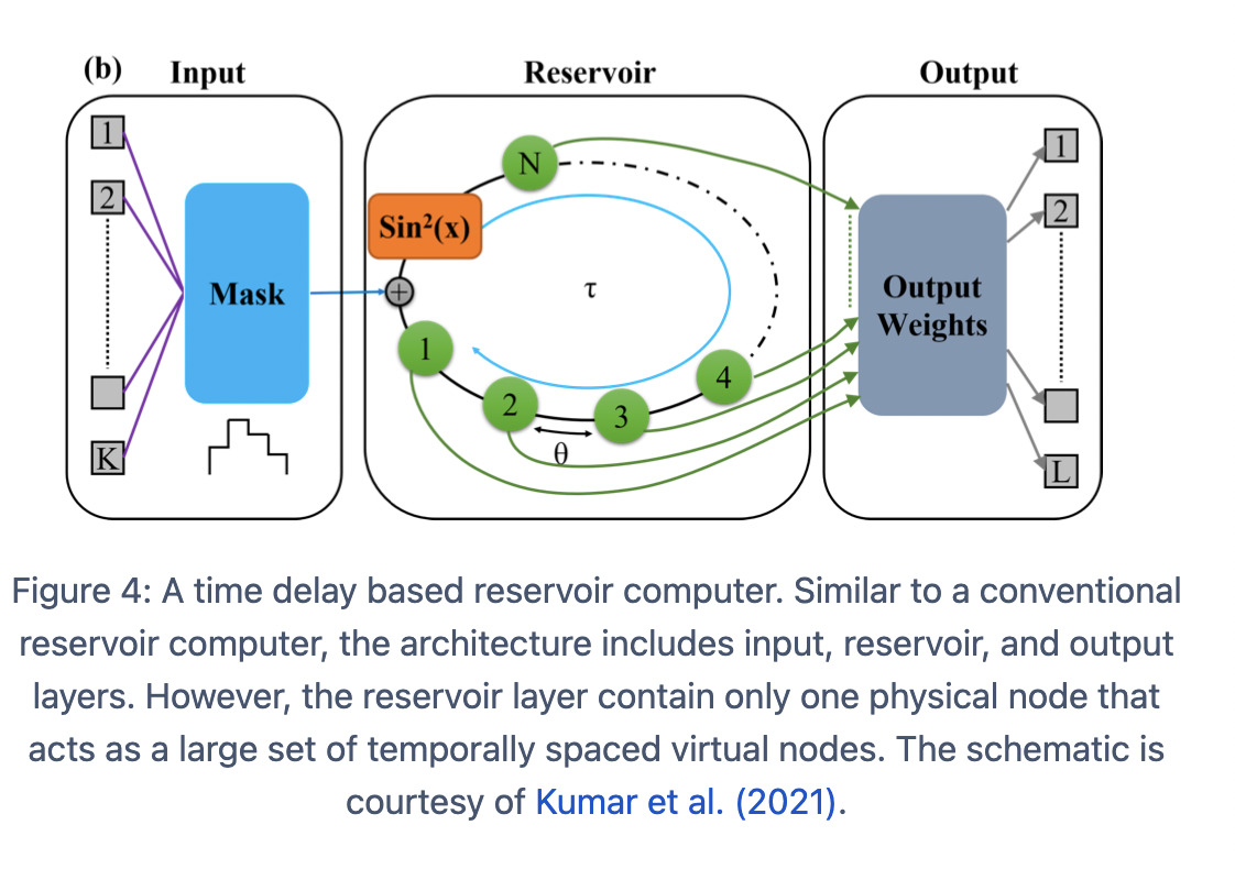
EmuCore, developed by QCi, represents a cutting-edge electronic reservoir computing platform designed specifically for tackling complex time series forecasting tasks. EmuCore harnesses the principles of reservoir computing, a powerful machine learning paradigm inspired by the brain’s dynamics, to efficiently process and predict time-dependent data. At the heart of EmuCore lies a large-scale dynamical system, referred to as the reservoir, composed of interconnected electronic components. These components exhibit rich nonlinear and chaotic dynamics, enabling EmuCore to capture and extract intricate patterns and dependencies present in time series data. The reservoir acts as a high-dimensional feature space where input signals are mapped and processed to generate accurate predictions. In this section, we explore the capabilities of EmuCore for time series forecasting tasks. We discuss the architecture and operation principles of EmuCore, highlighting its unique features and advantages. Furthermore, we demonstrate the effectiveness of EmuCore through practical examples and experiments, showcasing its ability to accurately predict complex time series data.
Through the integration of advanced hardware design, innovative algorithms, and rigorous testing, EmuCore represents a groundbreaking solution for time series forecasting and other machine learning tasks. Its versatility, performance, and efficiency make it a valuable tool for researchers, engineers, and practitioners seeking to push the boundaries of predictive analytics and intelligent systems.
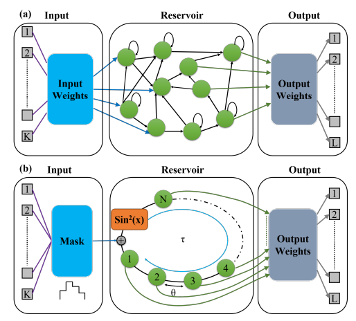
QCI’s EmuCore technology is based on a time delayed scheme. However, unlike other reservoir offerings from QCi the
 Photonic Reservoir Architecture and Benchmarking
Data Generation
Here we use widely used benchmark, namely NARMA10,
where the input 𝑢𝑘 is drawn from a uniform distribution in the interval .
The function below generates a NARMA10 time series and splits it into training and testing parts.
- import numpy as np
- def NARMA10(seed, train_size, test_size):
- np.random.seed(seed)
- total_size = train_size + test_size
- utrain = 0.5 * np.random.rand(total_size, 1)
- ytrain = np.zeros((10, 1))
- for i in list(range(9, total_size - 1)):
- temp = (
- 0.3 * ytrain[i]
- + 0.05 * ytrain[i] * np.sum(ytrain[i - 10 + 1 : i + 1])
- + 1.5 * utrain[i] * utrain[i - 10 + 1]
- + 0.1
- )
- ytrain = np.append(ytrain, [temp], axis=0)
- train_data = {
- "trainInput": utrain[0:train_size],
- "trainTarget": ytrain[0:train_size],
- }
- test_data = {
- "testInput": utrain[train_size:total_size],
- "testTarget": ytrain[train_size:total_size],
- }
- dataset = {"train_data": train_data, "test_data": test_data}
- return dataset
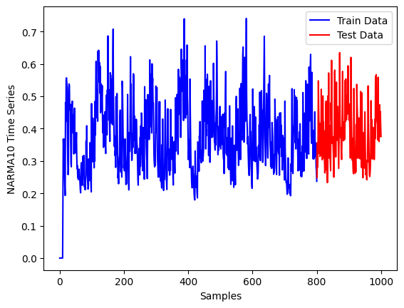
Let us consider a time series of size 1000 with 800 samples in the training part and 200 in the testing portiong.
- TRAIN_SIZE = 800
- TEST_SIZE = 200
- dataset = NARMA10(seed=0, train_size=TRAIN_SIZE, test_size=TEST_SIZE)
- X_train = dataset["train_data"]["trainInput"]
- y_train = dataset["train_data"]["trainTarget"].reshape((TRAIN_SIZE))
- X_test = dataset["test_data"]["testInput"]
- y_test = dataset["test_data"]["testTarget"].reshape((TEST_SIZE))
The target for this forecast is plotted below with the training portion in blue and the testing portion in red:
- import matplotlib.pyplot as plt
- t_train = np.linspace(0, TRAIN_SIZE, TRAIN_SIZE)
- t_test = np.linspace(TRAIN_SIZE, TRAIN_SIZE + TEST_SIZE, TEST_SIZE)
- plt.plot(t_train, y_train, "b")
- plt.plot(t_test, y_test, "r")
- plt.legend(["Train Data", "Test Data"])
- plt.xlabel("Samples")
- plt.ylabel("NARMA10 Time Series")
- plt.show()
Genearate Reservoir Output
After filling out some necessary details including replacing the IP_ADDR and PORT variables with our specific hardware destination we can begin interacting with the device through the client interface. Utilizing EmuCore’s direct interface we first begin by acquiring the lock. This ensures that the device is not being utilized by other users or processes and ensures that no one other than the current user can manipulate the reservoir anyway. Some of the ways we can interact with the hardware include resettign the reservoir and configuring reservoir size and attributes.
- from emucore_direct.client import EmuCoreClient
- from time import time
- IP_ADDR = "172.18.41.70"
- PORT = "50051"
- VBIAS = 0.31
- GAIN = 0.72
- NUM_NODES = 400
- NUM_TAPS = 400
- FEATURE_SCALING = 0.1
- DENSITY = 1.0
- # Instantiate an EmuCore instance
- ec_client = EmuCoreClient(ip_addr=IP_ADDR)
- # A a lock id and reset the device
- lock_id, start, end = ec_client.wait_for_lock()
---------------------------------------------------------------------------
_InactiveRpcError                         Traceback (most recent call last)
File ~/repos/emucore-direct/emucore_direct/client.py:153, in EmuCoreClient.acquire_lock(self)
    152 try:
--> 153     acquire_lock_resp = self.stub.acquire_lock(emucore_pb2.empty_message())
    154 except _InactiveRpcError as exc:

File ~/repos/emucore-direct/venv/lib/python3.10/site-packages/grpc/_channel.py:946, in _UnaryUnaryMultiCallable.__call__(self, request, timeout, metadata, credentials, wait_for_ready, compression)
    944 state, call, = self._blocking(request, timeout, metadata, credentials,
    945                               wait_for_ready, compression)
--> 946 return _end_unary_response_blocking(state, call, False, None)

File ~/repos/emucore-direct/venv/lib/python3.10/site-packages/grpc/_channel.py:849, in _end_unary_response_blocking(state, call, with_call, deadline)
    848 else:
--> 849     raise _InactiveRpcError(state)

_InactiveRpcError: <_InactiveRpcError of RPC that terminated with:
        status = StatusCode.UNAVAILABLE
        details = "failed to connect to all addresses"
        debug_error_string = "{"created":"@1711693535.063393946","description":"Failed to pick subchannel","file":"src/core/ext/filters/client_channel/client_channel.cc","file_line":3260,"referenced_errors":[{"created":"@1711693535.063391611","description":"failed to connect to all addresses","file":"src/core/lib/transport/error_utils.cc","file_line":167,"grpc_status":14}]}"
>

The above exception was the direct cause of the following exception:

InactiveRpcError                          Traceback (most recent call last)
Cell In[2], line 17
     14 ec_client = EmuCoreClient(ip_addr=IP_ADDR)
     16 # A a lock id and reset the device
---> 17 lock_id, start, end = ec_client.wait_for_lock()

File ~/repos/emucore-direct/emucore_direct/client.py:247, in EmuCoreClient.wait_for_lock(self)
    245 start_queue_ts = time.time_ns()
    246 while lock_id == "":
--> 247     lock_id = self.acquire_lock()["lock_id"]
    248     # only sleep if didn't get lock on device
    249     if lock_id == "":

File ~/repos/emucore-direct/emucore_direct/client.py:155, in EmuCoreClient.acquire_lock(self)
    153     acquire_lock_resp = self.stub.acquire_lock(emucore_pb2.empty_message())
    154 except _InactiveRpcError as exc:
--> 155     raise InactiveRpcError(
    156         "acquire_lock failed due to grpc._channel._InactiveRpcError."
    157     ) from exc
    158 return message_to_dict(acquire_lock_resp)

InactiveRpcError: acquire_lock failed due to grpc._channel._InactiveRpcError.
- VBIAS = 0.31
- GAIN = 0.72
- NUM_NODES = 400
- NUM_TAPS = 400
- FEATURE_SCALING = 0.1
- DENSITY = 1.0
- # A a lock id and reset the device
- #lock_id, start, end = client.wait_for_lock()
- print("Reservoir reset")
- ec_client.reservoir_reset(lock_id=lock_id)
- print("Reservoir config")
- # Configure
- ec_client.rc_config(
- lock_id=lock_id,
- vbias=VBIAS,
- gain=GAIN,
- num_nodes=NUM_NODES,
- num_taps=NUM_TAPS
- )
- #np.random.seed(10)
- #s=np.random.random(1, NUM_NODES , 0.5)
- #np.random.seed(10)
- #input_wgts=(2 * np.random.randint(low=0, high=2, size=(1, num_nodes)) - 1) * s.A
- print("Process job")
- # Push data through reservoir
- resp_train, train_max_scale_val, train_wgts = ec_client.process_all_data(
- input_data=X_train,
- num_nodes=NUM_NODES,
- density=DENSITY,
- feature_scaling=FEATURE_SCALING,
- lock_id=lock_id,
- #weights=input_wgts,
- #seed_val_weights = 10,
- #max_scale_val=None,
- )
- resp_test, test_max_scale_val, test_wgts = ec_client.process_all_data(
- input_data=X_test,
- num_nodes=NUM_NODES,
- density=DENSITY,
- feature_scaling=FEATURE_SCALING,
- lock_id=lock_id,
- #weights=input_wgts,
- #seed_val_weights = 10,
- #max_scale_val=None,
- )
Reservoir reset
Reservoir config
Process job
- ec_client.release_lock(lock_id=lock_id)
{'status': 0, 'message': 'Success'}
Build a Linear Model
Once we have the reservoir response, we can build a simple linear regression model using the reservoir response as its input.
- from sklearn.linear_model import LinearRegression
- from sklearn.metrics import mean_squared_error, r2_score
- #resp_train = np.load("resp_train.npy")
- #resp_test = np.load("resp_test.npy")
- lin_model = LinearRegression()
- lin_model.fit(resp_train, y_train)
- y_pred_train = lin_model.predict(resp_train)
- y_pred_test = lin_model.predict(resp_test)
- # Calculate Mean Squared Error and R-squared
- mse_train = mean_squared_error(y_train, y_pred_train)
- r2_train = r2_score(y_train, y_pred_train)
- print(f"Train Mean Squared Error: {mse_train:.4f}")
- print(f"Train R-squared: {r2_train:.2f}")
- mse_test = mean_squared_error(y_test, y_pred_test)
- r2_test = r2_score(y_test, y_pred_test)
- print(f"Test Mean Squared Error: {mse_test:.4f}")
- print(f"Test R-squared: {r2_test:.2f}")
Train Mean Squared Error: 0.0002
Train R-squared: 0.98
Test Mean Squared Error: 0.0004
Test R-squared: 0.95
We can look at the normalized root mean squared error (NRMSE), defined as,
- def NRMSE(target, estimate):
- return np.sqrt(((estimate - target) ** 2).mean()) / np.std(target)
- print(NRMSE(y_test, y_pred_test))
0.2247502186806958
- def StepPlotData(y1,y2,legend1="y1",legend2="y2"):
- plt.figure()
- assert(y1.shape[0]==y2.shape[0])
- i=np.arange(y1.shape[0])
- plt.step(i,y1,'r', where='mid', label=legend1,alpha=0.6)
- plt.legend()
- plt.step(i,y2,'g', where='mid', label=legend2,alpha=0.6)
- plt.legend()
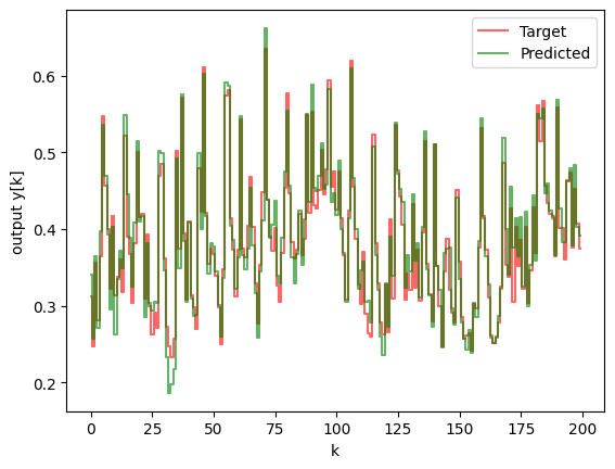
- StepPlotData(y1=y_test, y2=y_pred_test, legend1="Target", legend2="Predicted")
- plt.xlabel("k")
- plt.ylabel("output y[k]")
- #plt.figure()
- #plt.imshow(test_x, cmap="nipy_spectral")
- #plt.colorbar()
- plt.figure()
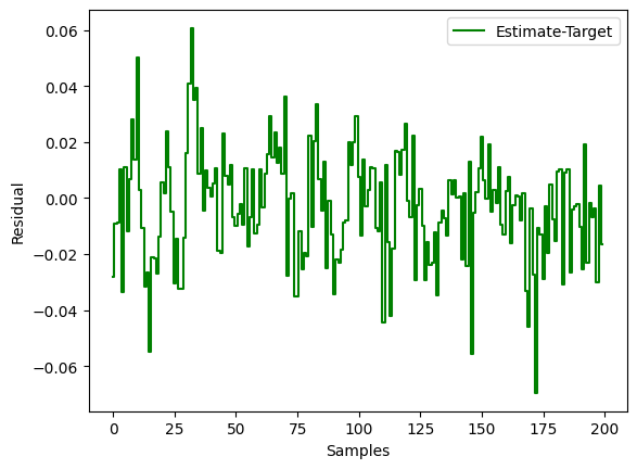
- plt.step(y_test-y_pred_test,'g', where='mid', label="Estimate-Target")
- plt.legend()
- plt.xlabel("Samples")
- plt.ylabel("Residual")
- plt.show()